Introduction to General Transit Feed Specifications (GTFS) with R
Introduction
The General Transit Feed Specification (GTFS) is a structured format for public transport data. This structured format allows public transport agencies to share their public transport information to write applications and build databases.
The GTFS is composed of different data tables related by id’s which makes them a relational database. These tables are stored in different .txt files in a .zip file. Each file mirrors the aspects of the public transport data like stops, routes, trips, and other schedule data. For more information Click here
The following image shows the common structure of a GTFS with different tables related by their respective id:
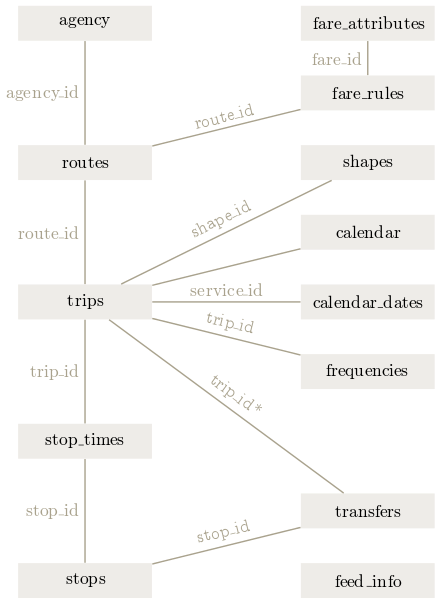
GTFS structure. Source: Wikimedia
At this Link, you will find the common .txt. files that make up a GTFS, their respective fields and the kind of data to be filled.
Start using tidytransit
We will take you through a simple example of the use of the “tidytransit” package. A simple and easy tool to handle a GTFS quickly and fast.
# First one you need to intall the tidytransit package considering it depends of package "sf"
# install.packages('tidytransit')

# Packages used
library(sf)
library(tidytransit)
library(leaflet)
library(dplyr)
Read GTFS in R
In this example, we will read a .zip file included in the self package to use it in the “read_gtfs”. This function will take the different .txt files and it will store them into a list object in R.
local_gtfs_path <- system.file("extdata",
                               "google_transit_nyc_subway.zip",
                               package = "tidytransit")
# Here you can put a URL or the folder path of your local machine
nyc <- read_gtfs(local_gtfs_path)

# A summary
summary(nyc)
## tidygtfs object
## files agency, stops, routes, trips, stop_times, calendar, calendar_dates, shapes, transfers
## agency MTA New York City Transit
## service from 2018-06-24 to 2018-11-03
## uses stop_times (no frequencies)
## # routes 29
## # trips 19890
## # stop_ids 1503
## # stop_names 380
## # shapes 215Now you can access the different tables by calling them in the “nyc” object
#Check out the stop table
head(nyc$stops)
## # A tibble: 6 x 10
## stop_id stop_code stop_name stop_desc stop_lat stop_lon zone_id stop_url
## <chr> <chr> <chr> <chr> <dbl> <dbl> <chr> <chr>
## 1 101 "" Van Cortlandt ~ "" 40.9 -73.9 "" ""
## 2 101N "" Van Cortlandt ~ "" 40.9 -73.9 "" ""
## 3 101S "" Van Cortlandt ~ "" 40.9 -73.9 "" ""
## 4 103 "" 238 St "" 40.9 -73.9 "" ""
## 5 103N "" 238 St "" 40.9 -73.9 "" ""
## 6 103S "" 238 St "" 40.9 -73.9 "" ""
## # ... with 2 more variables: location_type <int>, parent_station <chr>Validate GTFS
Tidytransit package includes a function to validate a GTFS by their required fields and files to verify the completeness
#Validate
validation_result <- attr(nyc, "validation_result")
head(validation_result)
## # A tibble: 6 x 8
## file file_spec file_provided_status field field_spec field_provided_~
## <chr> <chr> <lgl> <chr> <chr> <lgl>
## 1 agency req TRUE agency_id opt TRUE
## 2 agency req TRUE agency_name req TRUE
## 3 agency req TRUE agency_url req TRUE
## 4 agency req TRUE agency_time~ req TRUE
## 5 agency req TRUE agency_lang opt TRUE
## 6 agency req TRUE agency_phone opt TRUE
## # ... with 2 more variables: validation_status <chr>, validation_details <chr>Relate tables by ID
Considering the GTFS as a relational database, we can use functions from “dplyr” package (left_join, right_join) to join tables by an id common in two tables.
Let’s check out which days the routes operate
# Join tables by a common ID
StopsByRoute <- nyc$routes %>%
  left_join(nyc$trips, by = "route_id") %>%
  left_join(nyc$calendar, by = "service_id") %>%
  select(route_long_name,trip_headsign,monday, tuesday, wednesday, thursday, friday, saturday, sunday )

# Plt a sample of 1000 values
print(StopsByRoute[1:50,])
## # A tibble: 50 x 9
## route_long_name trip_headsign monday tuesday wednesday thursday friday
## <chr> <chr> <int> <int> <int> <int> <int>
## 1 Broadway - 7 Avenue L~ South Ferry 0 0 0 0 0
## 2 Broadway - 7 Avenue L~ South Ferry 0 0 0 0 0
## 3 Broadway - 7 Avenue L~ South Ferry 0 0 0 0 0
## 4 Broadway - 7 Avenue L~ South Ferry 0 0 0 0 0
## 5 Broadway - 7 Avenue L~ Van Cortland~ 0 0 0 0 0
## 6 Broadway - 7 Avenue L~ South Ferry 0 0 0 0 0
## 7 Broadway - 7 Avenue L~ Van Cortland~ 0 0 0 0 0
## 8 Broadway - 7 Avenue L~ South Ferry 0 0 0 0 0
## 9 Broadway - 7 Avenue L~ Van Cortland~ 0 0 0 0 0
## 10 Broadway - 7 Avenue L~ South Ferry 0 0 0 0 0
## # ... with 40 more rows, and 2 more variables: saturday <int>, sunday <int>Plot the GTFS spatial objects
There is a simple function called “gtfs_as_sf” to turn stops and shapes files into a simple feature object in R.
# Transform stops ans shapes ino a simple features
sfGtfs <- gtfs_as_sf(nyc, skip_shapes = FALSE, crs = NULL, quiet = TRUE)

# Create a palette of colors
pal <- colorFactor(
  palette = "viridis",
  domain = sfGtfs$shapes$shape_id)
# A leaflet map
mapa <- leaflet(sfGtfs$shapes)%>%
  addPolylines(color = ~pal(sfGtfs$shapes$shape_id),
               popup = sfGtfs$shapes$shape_id) %>%
  addTiles()%>%
  addProviderTiles("Stamen.TonerHybrid")

mapaHéctor Báez
Geologist Engineer
My research focuses on spatial data analysis, GIS, and web development to share knowledge of geospatial data.